Choosing what to throw away
Our paper in Scientific Reports on multi-label feature selection. Instead of picking the best features once, PG-GFE removes the weakest ones in stages and lets a graph decide what weak means.
Most feature selection works like a single decision. You score every feature, rank them, keep the top half, and hand the result to a classifier. The scoring happens once, against the full feature space, and whatever the score says at that moment is what you live with.
That assumption is the thing our paper takes apart. Once you remove a chunk of features, the remaining ones are no longer in the situation they were scored in. A feature that looked redundant only looked that way because a near-duplicate was sitting beside it. Remove the duplicate and the survivor becomes the only carrier of that signal. Its true value went up, but its score was written down before any of that happened, and nothing goes back to revise it.
The paper is Adaptive graph-evolutionary framework for dynamic feature refinement in multi-label learning, in Scientific Reports, with Hossien Movahed and Tina Toosi. The method is called PG-GFE, for Progressive Graph-Guided Feature Elimination.
Why multi-label makes this worse
In ordinary classification each instance gets one label. In multi-label learning it can carry many at once: a photograph tagged beach, sunset and people, a gene annotated with a dozen functions, a news article filed under several topics simultaneously.
Two things follow. Labels are correlated, so beach and sunset travel together and a feature that predicts one may be doing so only through the other. And feature relevance becomes label-specific: a feature can be indispensable for one label and pure noise for another. A single global score has to average over all of that, and averaging is exactly how you lose the structure that mattered.
The datasets make the scale concrete. Delicious carries 983 labels across 500 features. Corel5k has 374 labels. Bibtex has 1,836 features. Ranking those once and hoping is optimistic.
The idea
Treat feature reduction as a sequence of decisions rather than one decision.
At every stage, build a graph describing how features, labels and instances relate right now. Use it to work out which features are carrying reliable signal. Remove some of the weakest. Then rebuild the graph, because removing them changed the situation, and go again. Stop when the picture stops moving.
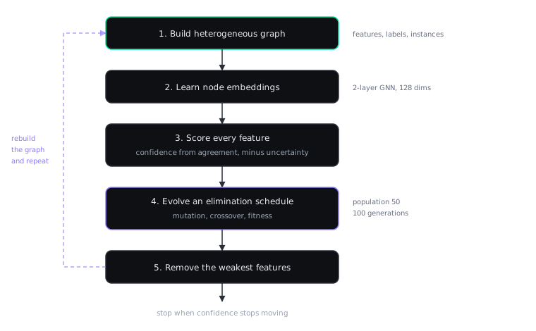
Nothing here is exotic on its own. Graph neural networks are well established, so is evolutionary optimization. What the paper argues is that the two belong in a closed loop: the graph produces a judgment about feature reliability, the evolutionary search decides how aggressively to act on it, and the consequences feed back into the next graph.
The graph
Three kinds of node, three kinds of edge.
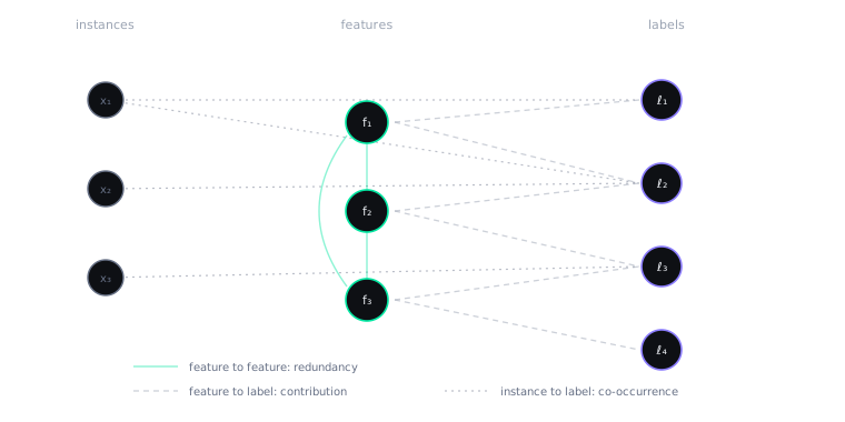
Feature-to-feature edges capture redundancy and complementarity: which features are saying the same thing. Feature-to-label edges capture contribution: how much a feature has to do with a particular label. Instance-to-label edges capture co-occurrence, which is where label correlation enters the model rather than being assumed away.
Keeping instances in the graph matters. Without them the model sees features and labels but not the evidence connecting them, and label correlation has to be imposed as a prior instead of being observed.
Confidence, and the part that does the real work
A graph neural network learns an embedding for every node. From those embeddings each feature gets a confidence score built from two terms.
The first is agreement: the average cosine similarity between a feature’s embedding and those of its neighbors. A feature sitting in a coherent neighborhood, pointing the same way as things it is genuinely related to, scores well.
The second is uncertainty, and this is the more interesting half. It is the variance of a feature’s association across all the labels. A feature that relates consistently to the labels it should relate to has low variance. A feature whose relationship swings wildly depending on which label you ask about has high variance, and gets penalized.
That distinction is what separates this from ordinary importance scoring. A feature can look important on average while being wildly inconsistent underneath. Averaging hides that. Variance surfaces it. The final confidence is agreement minus uncertainty, squashed into the range zero to one.
Scheduling the removals
Here is where it stops resembling normal feature selection. The evolutionary part does not search for the best feature subset. It searches for the best elimination schedule.
Each candidate solution is a binary mask over the features that survive at this stage: one means remove, zero means keep. Masks are seeded from the confidence scores, so a feature with confidence 0.2 has an 0.8 chance of being marked for removal in the initial population. Mutation and crossover then explore alternative removal patterns, and each candidate is judged on three things at once: how much predictive loss it caused, how much it destabilized confidence across the remaining features, and how many features it actually removed.
The mutation rate is deliberately front-loaded. It starts near 0.3 and decays toward 0.1 as stages progress, so the method is bold while there is plenty of redundancy to cut and cautious once the surviving set is lean. Anyone who has planned a staged rollout will recognize the shape of that: take the big, safe reductions early, slow down as the remaining margin shrinks.
Knowing when to stop
After each round of removals the graph is rebuilt and every confidence score is recomputed. The method then watches how much those scores moved, averaged across the surviving features.
Large movement means the last cut genuinely changed the structure and more care is needed. Movement approaching zero means the feature space has settled: what remains is stable under further pruning. That, together with a bound on performance drift, is the stopping condition. The output is not a subset chosen by a threshold, it is whatever the elimination trajectory converged on.
What was tested
Eight benchmark datasets from the Mulan and UCI repositories, spanning music, text, images, video and biology.
| Dataset | Instances | Features | Labels | Domain |
|---|---|---|---|---|
| Emotions | 593 | 72 | 6 | Music |
| Enron | 1,702 | 1,001 | 53 | Text |
| Scene | 2,407 | 294 | 6 | Image |
| Yeast | 2,417 | 103 | 14 | Biology |
| Bibtex | 7,395 | 1,836 | 159 | Text |
| Delicious | 16,105 | 500 | 983 | Text |
| Mediamill | 43,907 | 120 | 101 | Video |
| Corel5k | 5,000 | 499 | 374 | Image |
Two classifiers were used to check the result was not an artifact of one learner: MLkNN with k of 10, and Binary Relevance with a linear SVM. Ten independent runs each, stratified 10-fold cross-validation so every fold preserves the label distribution. Roughly half the original features were retained, and every competing method was given the same budget. PyTorch for the graph network, DEAP for the evolutionary search, population of 50 over 100 generations.
The comparison set was AKLS, MOD-DE, MG-GCN, JobXMLC, MLACO and FLSA-GRL: kernel-based, evolutionary, graph-based and swarm-based approaches, so the result is not measured against a single school of thought.
What the numbers say
Under MLkNN, against the strongest competing method on each dataset:
| Dataset | Hamming loss ↓ | Average precision ↑ | Ranking loss ↓ |
|---|---|---|---|
| Emotions | 0.175 vs 0.188 | 0.845 vs 0.828 | 0.115 vs 0.132 |
| Enron | 0.041 vs 0.043 | 0.682 vs 0.668 | 0.038 vs 0.049 |
| Scene | 0.072 vs 0.076 | 0.922 vs 0.915 | 0.035 vs 0.042 |
| Yeast | 0.168 vs 0.172 | 0.765 vs 0.752 | 0.112 vs 0.128 |
| Bibtex | 0.008 vs 0.009 | 0.518 vs 0.502 | 0.065 vs 0.076 |
| Delicious | 0.014 vs 0.015 | 0.372 vs 0.358 | 0.192 vs 0.208 |
| Mediamill | 0.033 vs 0.035 | 0.622 vs 0.608 | 0.082 vs 0.092 |
| Corel5k | 0.005 vs 0.006 | 0.292 vs 0.278 | 0.128 vs 0.142 |
The pattern held under Binary Relevance, which matters because BR deliberately tears the labels apart and treats each independently. A method that only worked when label correlation was modeled end to end would lose its advantage there.
Two honest observations about this table. The Hamming loss margins are small in absolute terms, sometimes a single thousandth, and on their own they would not be convincing. The ranking loss margins are the more meaningful result: 0.115 against 0.132 on Emotions, or 0.038 against 0.049 on Enron, are proportionally large. Ranking loss measures how often label pairs come back in the wrong order, so this is the metric most directly about label correlation, which is precisely what the method claims to preserve.
A Wilcoxon signed-rank test across all datasets returned p-values of 0.0078 for almost every comparison, comfortably below 0.05. The single exception was the F1-measure against FLSA-GRL at 0.0253: still significant, but noticeably closer, which is worth saying out loud rather than burying.
What it costs
The obvious objection to a method that repeats an expensive procedure many times is that it must be slow. Reported runtimes, in seconds:
| Dataset | PG-GFE | MLACO | AKLS | MOD-DE |
|---|---|---|---|---|
| Emotions | 8.9 | 10.3 | 12.5 | 18.2 |
| Enron | 38.5 | 42.6 | 45.3 | 52.1 |
| Bibtex | 82.4 | 88.7 | 95.2 | 112.5 |
| Mediamill | 245.1 | 265.8 | 280.4 | 325.7 |
Running the loop repeatedly turns out to be cheaper than the alternatives, because each pass operates on a smaller feature set than the one before. The first iteration is the expensive one and every subsequent iteration is cheaper. Reduction compounds in your favor.
Where it breaks
The paper is explicit about the limits, and they are worth repeating because they define where the method should not be reached for.
Memory. It depends on graph neural networks, so beyond roughly 100,000 instances memory consumption becomes the binding constraint. Past that point you need distributed training, which the paper does not address.
Imbalance. The evolutionary component assumes reasonably balanced label distributions. Severely skewed data, of the kind common in medical diagnostics where the interesting label is rare, is where this assumption is weakest.
Hyperparameters. The confidence balance and the elimination rate bounds need tuning per dataset. Values were fixed by grid search on a validation subset here, but a method needing per-dataset tuning is a method with an operational cost attached.
Why I find this interesting beyond the paper
The structure of PG-GFE is a control loop. Observe the system, form a judgment under uncertainty, act in a bounded way, observe the consequences, adjust. It is staged rollout with a stopping condition, applied to a feature space instead of a fleet.
The design decisions have the same shape too. Act aggressively while the blast radius is small and the redundancy is high. Slow down as the remaining margin shrinks. Never make an irreversible decision on a single observation. Treat instability as a signal in its own right rather than noise to average away. Stop when the measurements stop moving, not when a counter runs out.
I spend most of my time on infrastructure rather than machine learning, and what drew me to this problem was recognizing that reasoning. The interesting part of the paper is not that a graph neural network can score features. It is the argument that a single scoring pass is the wrong shape for the problem, because the thing being measured changes as you act on the measurement.
That is a familiar failure in operations. It turns out to be a failure in feature selection too.
Citation. Movahed, H., Toosi, T. & Nael, S. Adaptive graph-evolutionary framework for dynamic feature refinement in multi-label learning. Scientific Reports (2026). doi.org/10.1038/s41598-026-56255-5